Creating dynamic charts and graphs in spreadsheet software can help visualize data in a clear and concise manner. By incorporating interactive elements and automated updating features, you can easily showcase trends and patterns in your data. In this article, we will discuss how to create dynamic charts and graphs in popular spreadsheet software like Microsoft Excel and Google Sheets.
1. Choose the right data: Before creating a dynamic chart or graph, make sure to select the relevant data that you want to visualize. This data can be numerical values, percentages, or any other type of data that you want to represent graphically.
2. Insert a chart: In both Excel and Google Sheets, you can easily insert a chart by selecting the data range and choosing the desired chart type from the insert menu. Common chart types include bar graphs, line graphs, pie charts, and scatter plots.
3. Customize the chart: Once the chart is inserted, you can customize it by changing the chart style, colors, labels, and titles. You can also add data labels, trendlines, and other elements to make the chart more informative and visually appealing.
4. Make the chart dynamic: To make the chart dynamic, you can use features like data ranges and dynamic formulas. In Excel, you can use functions like OFFSET and named ranges to create dynamic charts that update automatically when new data is added.
5. Add interactivity: To enhance the user experience, you can add interactive elements to your chart, such as dropdown menus, buttons, or sliders. These elements can allow users to filter and analyze data dynamically, making the chart more engaging and informative.
By following these steps, you can create dynamic charts and graphs that effectively communicate your data and insights. Experiment with different chart types and customization options to find the best way to showcase your information visually.